
Introduction
This is the chapter web page to support the content in Chapter 8 of the book: Exploring BeagleBone – Tools and Techniques for Building with Embedded Linux. The summary introduction to the chapter is as follows:
This chapter describes bus communication in detail, explaining and comparing the different bus types that are available on the Beagle boards. It describes how you can configure them for use, and how you can communicate with and control I2C, SPI, and UART devices, using both Linux tools and custom-developed C/C++ code. Practical examples are provided using different low-cost bus devices, such as a real-time clock, an accelerometer, a serial shift register with a seven-segment display, a USB-to-TTL 3.3 V cable, and a GPS receiver. Finally, the AM335x DCAN controller is used to send and receive messages to and from a CAN Bus using Linux SocketCAN. After reading this chapter, you should have the skills necessary to begin interfacing almost any type of bus device to the Beagle boards.
Learning Outcomes
- Describe the most commonly used buses or interfaces that are available on the Beagle boards, and choose the correct bus to use for your application.
- Configure the Beagle boards to enable I2C, SPI, CAN bus, and UART capabilities.
- Attach circuits to a Beagle board that interface to its I2C bus, and use the Linux I2C-tools to communicate with those circuits.
- Build circuits that interface to the SPI bus using shift registers, and write C code that controls low-level SPI communication.
- Write C/C++ code that interfaces to and “wraps” the functionality of devices attached to the I2C and SPI buses.
- Communicate between UART devices using both Linux tools and custom C code.
- Build a basic distributed system that uses UART connections to the board to allow it to be controlled from a desktop PC.
- Interface to a low-cost GPS sensor using a UART connection.
- Build circuits that interface to the Beagle board CAN buses and use Linux SocketCAN to send and receive messages to and from the bus.
- Add logic-level translation circuitry to your circuits in order to communicate between devices with different logic-level voltages.
Digital Media Resources
Additional Content (for First Edition)
SPI Analog to Digital Converter (ADC) Example
- It deals with writing and reading to/from an SPI device. The ADXL345 SPI example in the book focuses on reading/writing register values. While it is essentially the same thing, different class methods are required for this example.
- This example is useful for communicating with SPI devices that have custom communication protocols.
- The MCP3008 is a very low-cost device that is widely available (in PDIP form).
- Chapter 6 describes how easy it is to damage the BeagleBone’s on-board Analog-to-Digital Converter (ADC) and therefore an external ADC might be preferable for some readers (e.g., the external ADC can easily be used with 3.3V levels). An external ADC also allows for the expansion of the total number of ADCs that are available on the BeagleBone.
For this example, the MCP3008 is used in a PDIP package (see the datasheet) – it is a low-cost, 8-channel 10-bit ADC with an SPI interface that can be powered at 3.3V. This particular IC can capture 75,000 samples per second when powered at 2.7V and 200,000 samples per second when powered at 5V – therefore the raw performance when powered at 3.3V is somewhere within this range. However, it does not appear possible to achieve the upper level of performance under a regular Linux kernel with the configuration that is proposed. There are many similar SPI ADCs (and indeed DACs), including the MCP3004 that has four 10-bit input channels, the MCP3204 that has four 12-bit channels, and the MCP3208 that has eight 12-bit channels. The code that is presented in this section can be easily adapted to support any of these devices.
There is a BeagleBone ADC Cape available from CircuitCo that has a MCP3008 and can be used with this example code.
In addition to eight independent single-ended inputs, the MCP3008 (and most of the extended family) support pseudo-differential input pairs. For example, CH0 can be used as IN+ and CH1 can be used as IN- and the difference between the two inputs can be determined. In this mode, the IN+ input can range from IN- (a zero value digital output) to the sum of Vref plus IN- (a digital output of 1023).
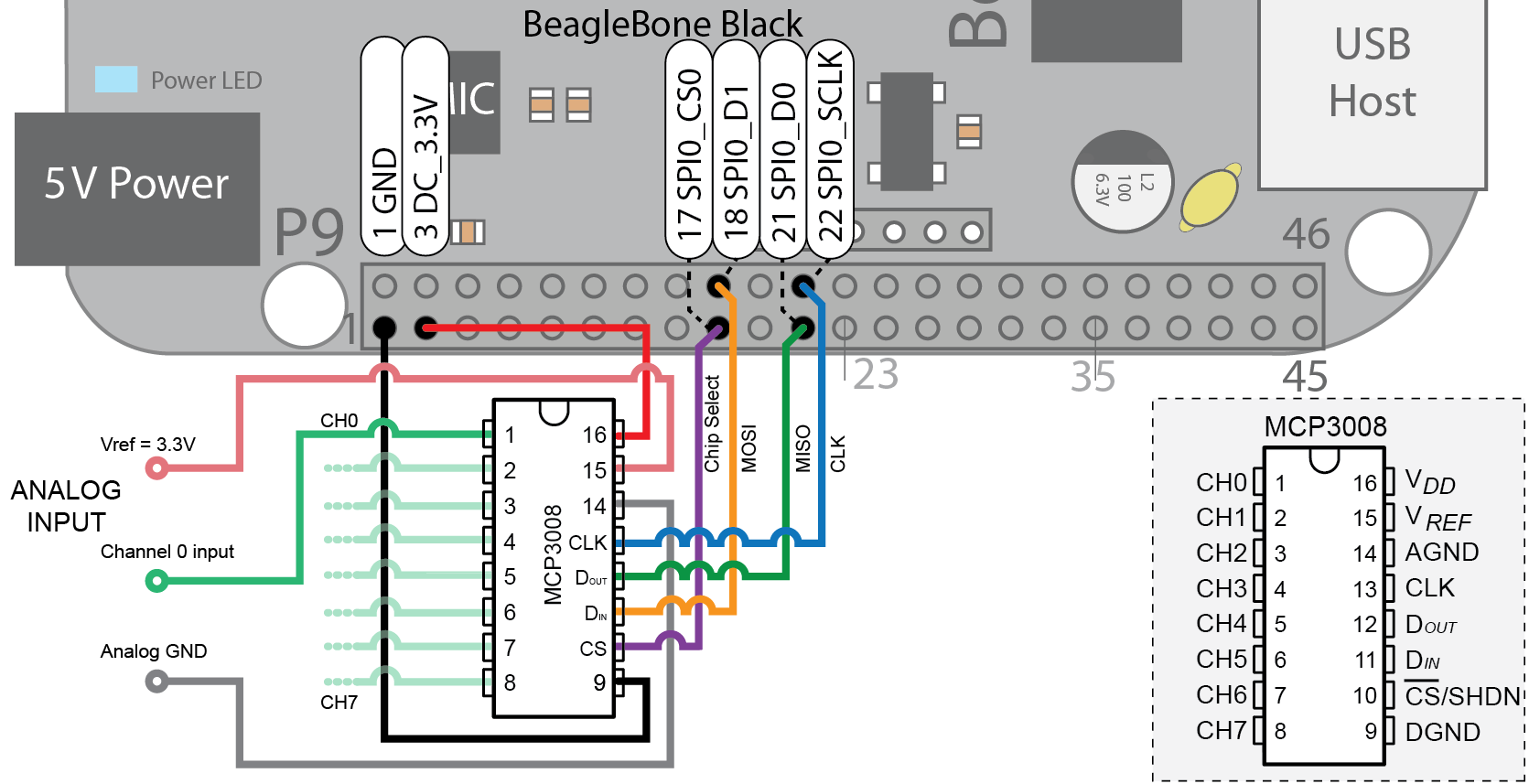
Figure 8.A1 The BeagleBone SPI ADC circuit
Figure 8.A1 illustrates how you can connect the SPI ADC to the BeagleBone Black using the pin configuration that is described in Table 8.A1 below. The Vref pin in Figure 8.A1 does not have to be set at 3.3V, however it is a useful initial range. For further information on the input characteristics study the datasheet.
Table 8.A1 Table of pin inputs/outputs for the 16-pin MCP3008.
| IC Pins | Pin Title | Description |
| Pins 1-8 | CH0-CH7 | The eight ADC inputs |
| Pin 9 | DGND | Digital ground – connected to the internal digital ground. Can be connected to the BBB GND. |
| Pin 10 | CS/SHDN | Chip Select/Shutdown. Used to initiate communication with the device when pulled low. When pulled high it “ends the conversation” and puts the device in standby. Must be pulled high between conversions. |
| Pin 11 | DIN | Used to transfer data that is used configure the converter (e.g., chose which ADC input to use and whether to use single-ended or differential inputs) |
| Pin 12 | DOUT | The SPI serial data output provides the results of the analog to digital conversion. The data bit changes on the falling edge of the clock. |
| Pin 13 | CLK | The SPI clock can be used to clock out the bits. Ideally a minimum clock rate of 10KHz should be maintained to avoid introducing linearity errors. |
| Pin 14 | AGND | Analog ground – connected to the internal analog circuit GND. |
| Pin 15 | VREF | Reference voltage input |
| Pin 16 | VDD | Voltage Supply (2.7V to 5.5V). Can be connected directly to the BBB 3.3V supply rail. |
Table 8.A2 Configuration of the operation mode for the MCP3008.
| Single-Ended Configuration (Single/Diff = 1) | Differential Configuration (Single/Diff = 0) | ||||||
| Control Bit Selections | Control Bit Selections | ||||||
| Channel | D2 | D1 | D0 | Channel | D2 | D1 | D0 |
| CH0 | 0 | 0 | 0 | IN+=CH0 IN-=CH1 | 0 | 0 | 0 |
| CH1 | 0 | 0 | 1 | IN+=CH1 IN-=CH0 | 0 | 0 | 1 |
| CH2 | 0 | 1 | 0 | IN+=CH2 IN-=CH3 | 0 | 1 | 0 |
| CH3 | 0 | 1 | 1 | IN+=CH3 IN-=CH2 | 0 | 1 | 1 |
| CH4 | 1 | 0 | 0 | IN+=CH4 IN-=CH5 | 1 | 0 | 0 |
| CH5 | 1 | 0 | 1 | IN+=CH5 IN-=CH4 | 1 | 0 | 1 |
| CH6 | 1 | 1 | 0 | IN+=CH6 IN-=CH7 | 1 | 1 | 0 |
| CH7 | 1 | 1 | 1 | IN+=CH7 IN-=CH6 | 1 | 1 | 1 |
The source code example below uses the SPI class that is described in Chapter 8. This example uses a Single-Ended Configuration, therefore Single/Diff=1 and the left-hand side of Table 8.A2 is used. As also described in the table, to sample from Channel CH0, the D2, D1, and D0 values must be set to 0. Therefore, the bit pattern to be sent to the ADC input in this case is 1000. In the code example provided below, these bits are set as the most-significant bits of send[1]. The last bit in send[0] is 1, which acts as the start bit to inform the device that a sample is being requested. The full code example is in the directory /chp08/spi/adc_example/
/* Using an SPI ADC (e.g., the MCP3008)
* Written by Derek Molloy for the book "Exploring BeagleBone: Tools and
* Techniques for Building with Embedded Linux" by John Wiley & Sons, 2014
* ISBN 9781118935125. Please see the file README.md in the repository root
* directory for copyright and GNU GPLv3 license information.            */

#include <iostream>
#include <sstream>
#include "bus/SPIDevice.h"

using namespace std;
using namespace exploringBB;

short combineValues(unsigned char upper, unsigned char lower){
   return ((short)upper<<8)|(short)lower;
}

int main(){
   cout << "Starting EBB SPI ADC Example" << endl;
   SPIDevice *busDevice = new SPIDevice(1,0); //Using second SPI bus (both loaded)
   busDevice->setSpeed(4000000);      // Have access to SPI Device object
   busDevice->setMode(SPIDevice::MODE0);

   unsigned char send[3], receive[3];
   send[0] = 0b00000001; // The Start Bit followed
   // Set the SGL/Diff and D mode -- e.g., 1000 means single ended CH0 value
   send[1] = 0b10000000; // The MSB is the Single/Diff bit and it is followed by 000 for CH0
   send[2] = 0;          // This byte doesn't need to be set, just for a clear display
   busDevice->transfer(send, receive, 3);
   cout << "Response bytes are " << (int)receive[1] << "," << (int)receive[2] << endl;

   // Use the 8-bits of the second value and the two LSBs of the first value
   int value = combineValues(receive[1]&0b00000011, receive[2]);
   cout << "This is the value " << value << " out of 1024." << endl;
   cout << "End of EBB SPI ADC Example" << endl;
}
This example can be executed and will give the output as follows:
root@beaglebone:/lib/firmware# echo BB-SPIDEV0 > $SLOTS
root@beaglebone:/lib/firmware# cat $SLOTS
 0: 54:PF---
 1: 55:PF---
 2: 56:PF---
 3: 57:PF---
 4: ff:P-O-L Bone-LT-eMMC-2G,00A0,Texas Instrument,BB-BONE-EMMC-2G
 5: ff:P-O-- Bone-Black-HDMI,00A0,Texas Instrument,BB-BONELT-HDMI
 6: ff:P-O-- Bone-Black-HDMIN,00A0,Texas Instrument,BB-BONELT-HDMIN
 7: ff:P-O-L Override Board Name,00A0,Override Manuf,BB-SPIDEV0

root@beaglebone:~/exploringBB/chp08/spi/adc_example# ./ADCExample
Starting EBB SPI ADC Example
Response value is 249 235
This is the value 491 out of 1024.
End of EBB SPI ADC Example
root@beaglebone:~/exploringBB/chp08/spi/adc_example#
This will give the output on the Logic Analyzer as in Figure 8.A2 below. In this figure you can see that the values which are sent to the SPI ADC are 0x01 followed by 0x80 (and a blank value of 0x00) on the MOSI line (orange). The SPI ADC responds on the MISO line (green) with the value 0xF9 and 0xEB. These values are 0xF9 = 249 decimal and 0xEB = 235 decimal in the code example output above. This data needs to be parsed to extract the actual ADC response value. This is achieved by taking the last two bits of the first byte (0xF9 = 0b11111001) and all eight bits of the second byte (0xEB = 0b11101011) in order to create the binary value 0b0111101011, which is 491 decimal (as outputted by the code example above).
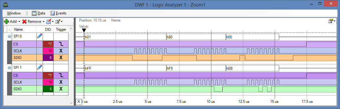
Figure 8.A2 The Logic Analyzer output for the code example above (note: the colors align with the connection wires in Figure 8.A1)
Adapting this Example for the 12-bit MCP3204/08
To adapt this code for the 12-bit MCP3204/08 (see the datasheet) you need to make a few modifications to the source code. The circuit has the exact same wiring configuration as in Figure 8.A1 and uses a very similar structure. The significant difference in the configuration relates to Figure 6-1 in both datasheets. Since there are an additional 2 bits required for a MCP320x data transaction, the Start Bit and Data Channel selection bits are shifted left by two bits. Therefore, to complete a request for a single-ended sample from Channel 0 you must send the value 00000110 00xxxxxx xxxxxxxx = 0x060000. Therefore, send[0] = 0b00000110, and send[1] = send[2] =0. The response is now the 8-bits of receive[2] and the four LSBs of receive[1]. Therefore, the combineValues() function should be called as follows:
int value = combineValues(receive[1]&0b00001111, receive[2]);
which results in a 12-bit return value, so the result should be presented as “out of 4096”.
Gnuplot
molloyd@beaglebone:~$ sudo apt-get install gnuplot gnuplot-x11
Make sure that you install gnuplot-x11 if you are planning to display the output on screen. In the following example I am using a VNC connection to the BeagleBone — such a configuration is described in detail in the book at the beginning of Chapter 11. You can see that I use ssh -XC on my Linux desktop machine to connect to the BeagleBone for this very reason.
Once gnuplot is installed, you can test it using the following steps:
molloyd@debian:~$ ssh -XC molloyd@192.168.7.2
Debian GNU/Linux 7
BeagleBoard.org BeagleBone Debian Image 2014-05-14
Support/FAQ: http://elinux.org/Beagleboard:BeagleBoneBlack_Debian
molloyd@192.168.7.2's password:
molloyd@beaglebone:~$ gnuplot
	G N U P L O T
	Version 4.6 patchlevel 0    last modified 2012-03-04
	Build System: Linux armv7l
	Copyright (C) 1986-1993, 1998, 2004, 2007-2012
	Thomas Williams, Colin Kelley and many others
	gnuplot home:     http://www.gnuplot.info
	faq, bugs, etc:   type "help FAQ"
	immediate help:   type "help"  (plot window: hit 'h')
Terminal type set to 'wxt'
gnuplot> plot sin(x)
This should result in the on-screen display of a plot of sin(x) as in Figure 8.A3 below.
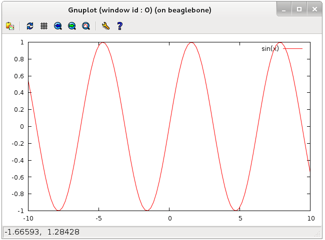
Figure 8.A3 Testing the gnuplot program
Gnuplot can also be used to output a print-ready or raster version of the plot in a file. In the following code segment the function is plotted to a PostScript file and to a PNG file. The PostScript file is subsequently converted to a PDF file using the ps2pdf tool so that it is more generally viewable, while remaining in a vector-mapped format.
molloyd@beaglebone:~$ gnuplot
...
gnuplot> set term postscript
Terminal type set to 'postscript'
Options are 'landscape noenhanced defaultplex ...
gnuplot> set output "test.ps"
gnuplot> plot sin(x)
gnuplot> set term png
Terminal type set to 'png'
Options are 'nocrop font ...
gnuplot> set output "test.png"
gnuplot> replot
gnuplot> set term x11
Terminal type set to 'x11'
gnuplot> replot
Closing test.png
gnuplot> exit
molloyd@beaglebone:~$ ls test.*
test.png test.ps
molloyd@beaglebone:~$ ps2pdf test.ps test.pdf
For your information, the outputted files are available here for you to view: test.png (5.41KB), test.pdf (3.78KB).
In the next section gnuplot is used to display the output from the ADC circuit that is used to sample a signal for a number of samples (200 and 20,000). To use gnuplot to plot your own data, you can simply pass the name of a file to gnuplot that contains a single data sample on each new line — this is demonstrated in the example in the next sectionFor more information on gnuplot, please see: www.gnuplot.info
SPI ADC with Multiple Samples
root@beaglebone:~/exploringBB/chp08/spi/adc_example# ./ADCmulti > data
root@beaglebone:~/exploringBB/chp08/spi/adc_example# echo 'plot "data" with linespoints lc rgb "blue"; pause 10' | gnuplot
root@beaglebone:~/exploringBB/chp08/spi/adc_example# echo 'set term postscript; set output "plot.ps"; plot "data" with linespoints lc rgb "blue";' | gnuplot
root@beaglebone:~/exploringBB/chp08/spi/adc_example# ls *.ps
plot.ps
root@beaglebone:~/exploringBB/chp08/spi/adc_example# ps2pdf plot.ps plot.pdf
A sine wave is applied to the ADC input using the Analog Discovery Waveform Generator in order to test the quality of the analog data capture. The 200 samples that are captured using the test application are plotted in Figure 8.A4 for different input sine wave signal frequencies of 50Hz, 500Hz, 1KHz, 2KHz, and 5KHz (moving left to right — click each image for a larger view).
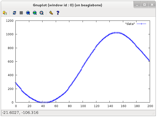
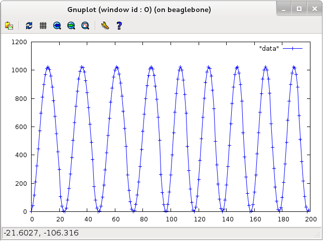
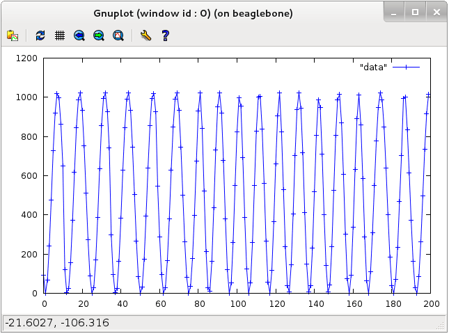
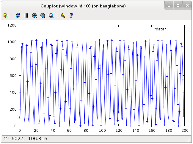
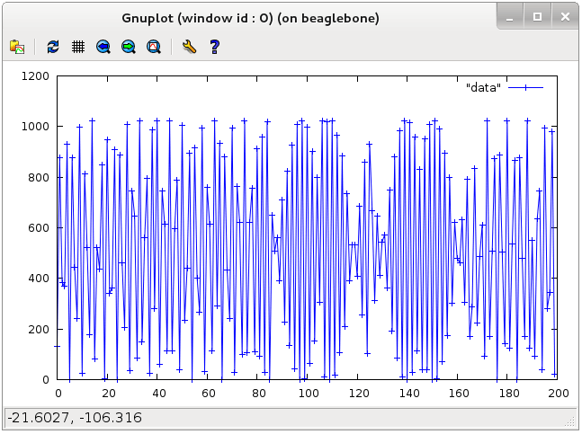
Figure 8.A4 (a)-(f) The ADCmulti application output displaying 200 samples from an input signal that varies from 50Hz to 5KHz.
A PDF version of the output at 500Hz is available in the file: plot.pdf. The circuit set up works surprisingly well up until the 2KHz sine wave is applied as the input. There are modest levels of jitter — however, that would not be the case for a longer sample duration at high frequencies, as the ADCmulti program is heavy on BeagleBone CPU resources.
This discussion also brings up an interesting point! The use of the BeagleBone frequency utilities is described in Chapter 5 (Page 153) and it is important to note that the CPU frequency of the BeagleBone has an impact on the performance of this application. For example, if the application is modified to take 20,000 samples and executed you will get a plot like this: Plot for On-Demand Governor (Also see Figure 8.A5 on the left-hand side). You can clearly see that there is a change in the observed frequency (after approximately 5,000 samples) — this is because the on-demand governor switches the BeagleBone CPU frequency to 1000MHz when the CPU is busy for an extended period.
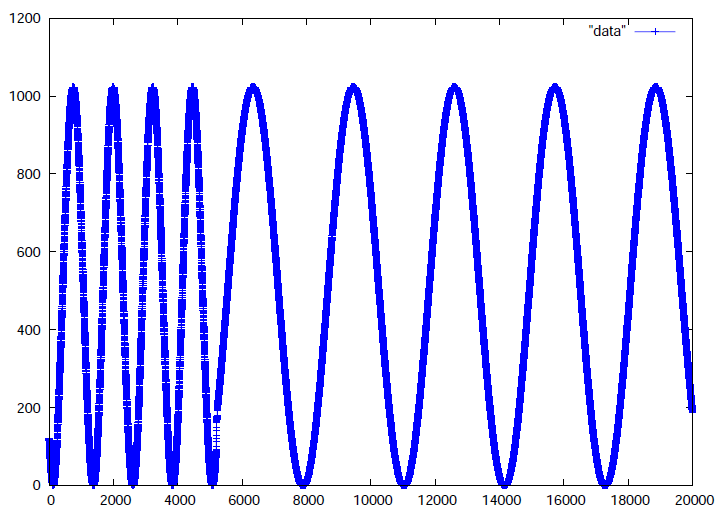
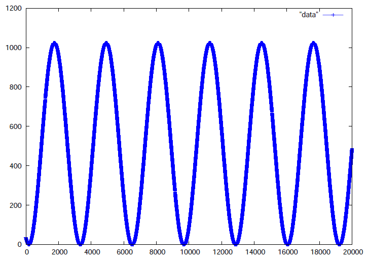
Figure 8.A5 (a) The ADCmulti application running with an “on demand” governor and (b) with a “performance” governor.
You can resolve this problem by setting the governor and re-capturing the data as follows:
root@beaglebone:~/exploringBB/chp08/spi/adc_example# cpufreq-set -g performance
root@beaglebone:~/exploringBB/chp08/spi/adc_example# ./ADCmulti2 > data
root@beaglebone:~/exploringBB/chp08/spi/adc_example# echo 'set term postscript; set output "plot.ps"; plot "data" with linespoints lc rgb "blue";' | gnuplot
root@beaglebone:~/exploringBB/chp08/spi/adc_example# ps2pdf plot.ps plot.pdf
The PDF plot of the output is now consistent and appears like this: Plot for Performance Governor (See Figure 8.A5 on the right-hand side).
If required, you can set the governor back to “on demand” using:
root@beaglebone:~/exploringBB/chp08/spi/adc_example# cpufreq-set -g ondemand
BeagleBone Bus Videos
An I²C Tutorial Video
In this video I discuss the I²C bus and how we can connect and program devices attached to the bus using C/C++. I explain the use of i2c-tools on embedded Linux and then show how we can interface to a digital accelerometer (Bosch BMA180) or any other I²C device. Finally, I show how we can use sysfs to build a C++ class that wraps the functionality of the digital accelerometer.

Arduino Videos
An Introduction to the Arduino
This is a short introduction to the Arduino platform.


An Arduino on a Breadboard
This tutorial shows you how to build an Arduino on a breadboard. It describes the use of 16MHz and 20Mhz crystals for driving the Arduino and compares their use to the use of a resonator. A simple circuit is created that blinks an LED for 1000ms and 100ms. The Arduino is programmed on the breadboard using an Arduino shield’s Reset, TX and RX pins.
LCD Display Introduction
This short video looks at the different options available for connecting an LCD character display to an Arduino. It uses a wide set of displays: The nuelectronics display shield, 20×4, 20×2,16×2 and 8×2 display modules. It shows the code that you need to create an example display and describes the use of the POT in the display. The modules used are the nuelectronics display shield, JHD 204, WH1602, CM200200 and a YJ 802A.


Arduino Application – A Reaction Timer
In this video I combine three previous videos and write some code to create an Arduino based Reaction Timer. The entire circuit is built on a breadboard using an ATmega328P on its own, which is combined with a Newhaven Display LCD Module that has an RGB backlight. I work through the code in some detail and explain how to write the code for the reaction timer. At the end of the video I provide links to the previous videos that show how to build the three individual circuits: Breadboard PSU, Arduino on a Breadboard and Arduino LCD Tutorial.
8×8 LED Dot Matrix Display Tutorial
In this video a 2 Colour (red/green) 8×8 LED Dot Matrix Display circuit is developed that uses three 74HC595 ICs to drive the rows/columns and a darlington transistor array (UDN2981A) to source the current. An Arduino is used to provide the serial data and the source code is presented to show how this was achieved. The display is a common anode display and the experiment spends time examining the current constraints, explaining why we require transistor arrays to source or sink current.

Source Code
You can clone this repository on a Linux desktop computer or your BeagleBone using the command:
git clone https://github.com/derekmolloy/exploringBB.git
The code for this chapter can be accessed in the chp08 folder of the cloned repository. The formatted code is provided here for your convenience.
I2CDevice.h
/*
 * I2C.h  Created on: 17 May 2014
 * Copyright (c) 2014 Derek Molloy (www.derekmolloy.ie)
 * Made available for the book "Exploring BeagleBone"
 * See: www.exploringbeaglebone.com
 * Licensed under the EUPL V.1.1
 *
 * This Software is provided to You under the terms of the European
 * Union Public License (the "EUPL") version 1.1 as published by the
 * European Union. Any use of this Software, other than as authorized
 * under this License is strictly prohibited (to the extent such use
 * is covered by a right of the copyright holder of this Software).
 *
 * This Software is provided under the License on an "AS IS" basis and
 * without warranties of any kind concerning the Software, including
 * without limitation merchantability, fitness for a particular purpose,
 * absence of defects or errors, accuracy, and non-infringement of
 * intellectual property rights other than copyright. This disclaimer
 * of warranty is an essential part of the License and a condition for
 * the grant of any rights to this Software.
 *
 * For more details, see http://www.derekmolloy.ie/
 */

#ifndef I2C_H_
#define I2C_H_
#include"BusDevice.h"

#define BBB_I2C_0 "/dev/i2c-0"
#define BBB_I2C_1 "/dev/i2c-1"

namespace exploringBB{

/**
 * @class I2CDevice
 * @brief Generic I2C Device class that can be used to connect to any type of I2C device and read or write to its registers
 */
class I2CDevice:public BusDevice{

public:
	I2CDevice(unsigned int bus, unsigned int device);
	virtual int open();
	virtual int write(unsigned char value);
	virtual unsigned char readRegister(unsigned int registerAddress);
	virtual unsigned char* readRegisters(unsigned int number, unsigned int fromAddress=0);
	virtual int writeRegister(unsigned int registerAddress, unsigned char value);
	virtual void debugDumpRegisters(unsigned int number = 0xff);
	virtual void close();
	virtual ~I2CDevice();
};

} /* namespace exploringBB */

#endif /* I2C_H_ */
I2CDevice.cpp
/*
 * I2C.cpp  Created on: 17 May 2014
 * Copyright (c) 2014 Derek Molloy (www.derekmolloy.ie)
 * Made available for the book "Exploring BeagleBone"
 * See: www.exploringbeaglebone.com
 * Licensed under the EUPL V.1.1
 *
 * This Software is provided to You under the terms of the European
 * Union Public License (the "EUPL") version 1.1 as published by the
 * European Union. Any use of this Software, other than as authorized
 * under this License is strictly prohibited (to the extent such use
 * is covered by a right of the copyright holder of this Software).
 *
 * This Software is provided under the License on an "AS IS" basis and
 * without warranties of any kind concerning the Software, including
 * without limitation merchantability, fitness for a particular purpose,
 * absence of defects or errors, accuracy, and non-infringement of
 * intellectual property rights other than copyright. This disclaimer
 * of warranty is an essential part of the License and a condition for
 * the grant of any rights to this Software.
 *
 * For more details, see http://www.derekmolloy.ie/
 */

#include"I2CDevice.h"
#include<iostream>
#include<sstream>
#include<fcntl.h>
#include<iomanip>
#include<stdio.h>
#include<unistd.h>
#include<sys/ioctl.h>
#include<linux/i2c.h>
#include<linux/i2c-dev.h>
using namespace std;

#define HEX(x) setw(2) << setfill('0') << hex << (int)(x)

namespace exploringBB {

/**
 * Constructor for the I2CDevice class. It requires the bus number and device number. The constructor
 * opens a file handle to the I2C device, which is destroyed when the destructor is called
 * @param bus The bus number. Usually 0 or 1 on the BBB
 * @param device The device ID on the bus.
 */
I2CDevice::I2CDevice(unsigned int bus, unsigned int device):
	BusDevice(bus,device){
	this->open();
}

/**
 * Open a connection to an I2C device
 * @return 1 on failure to open to the bus or device, 0 on success.
 */
int I2CDevice::open(){
   string name;
   if(this->bus==0) name = BBB_I2C_0;
   else name = BBB_I2C_1;

   if((this->file=::open(name.c_str(), O_RDWR)) < 0){
      perror("I2C: failed to open the bus\n");
	  return 1;
   }
   if(ioctl(this->file, I2C_SLAVE, this->device) < 0){
      perror("I2C: Failed to connect to the device\n");
	  return 1;
   }
   return 0;
}

/**
 * Write a single byte value to a single register.
 * @param registerAddress The register address
 * @param value The value to be written to the register
 * @return 1 on failure to write, 0 on success.
 */

int I2CDevice::writeRegister(unsigned int registerAddress, unsigned char value){
   unsigned char buffer[2];
   buffer[0] = registerAddress;
   buffer[1] = value;
   if(::write(this->file, buffer, 2)!=2){
      perror("I2C: Failed write to the device\n");
      return 1;
   }
   return 0;
}

/**
 * Write a single value to the I2C device. Used to set up the device to read from a
 * particular address.
 * @param value the value to write to the device
 * @return 1 on failure to write, 0 on success.
 */
int I2CDevice::write(unsigned char value){
   unsigned char buffer[1];
   buffer[0]=value;
   if (::write(this->file, buffer, 1)!=1){
      perror("I2C: Failed to write to the device\n");
      return 1;
   }
   return 0;
}

/**
 * Read a single register value from the address on the device.
 * @param registerAddress the address to read from
 * @return the byte value at the register address.
 */
unsigned char I2CDevice::readRegister(unsigned int registerAddress){
   this->write(registerAddress);
   unsigned char buffer[1];
   if(::read(this->file, buffer, 1)!=1){
      perror("I2C: Failed to read in the value.\n");
      return 1;
   }
   return buffer[0];
}

/**
 * Method to read a number of registers from a single device. This is much more efficient than
 * reading the registers individually. The from address is the starting address to read from, which
 * defaults to 0x00.
 * @param number the number of registers to read from the device
 * @param fromAddress the starting address to read from
 * @return a pointer of type unsigned char* that points to the first element in the block of registers
 */
unsigned char* I2CDevice::readRegisters(unsigned int number, unsigned int fromAddress){
	this->write(fromAddress);
	unsigned char* data = new unsigned char[number];
    if(::read(this->file, data, number)!=(int)number){
       perror("IC2: Failed to read in the full buffer.\n");
	   return NULL;
    }
	return data;
}

/**
 * Method to dump the registers to the standard output. It inserts a return character after every
 * 16 values and displays the results in hexadecimal to give a standard output using the HEX() macro
 * that is defined at the top of this file. The standard output will stay in hexadecimal format, hence
 * the call on the last like.
 * @param number the total number of registers to dump, defaults to 0xff
 */

void I2CDevice::debugDumpRegisters(unsigned int number){
	cout << "Dumping Registers for Debug Purposes:" << endl;
	unsigned char *registers = this->readRegisters(number);
	for(int i=0; i<(int)number; i++){
		cout << HEX(*(registers+i)) << " ";
		if (i%16==15) cout << endl;
	}
	cout << dec;
}

/**
 * Close the file handles and sets a temporary state to -1.
 */
void I2CDevice::close(){
	::close(this->file);
	this->file = -1;
}

/**
 * Closes the file on destruction, provided that it has not already been closed.
 */
I2CDevice::~I2CDevice() {
	if(file!=-1) this->close();
}

} /* namespace exploringBB */
SPIDevice.h
/*
 * SPIDevice.h  Created on: 22 May 2014
 * Copyright (c) 2014 Derek Molloy (www.derekmolloy.ie)
 * Made available for the book "Exploring BeagleBone"
 * See: www.exploringbeaglebone.com
 * Licensed under the EUPL V.1.1
 *
 * This Software is provided to You under the terms of the European
 * Union Public License (the "EUPL") version 1.1 as published by the
 * European Union. Any use of this Software, other than as authorized
 * under this License is strictly prohibited (to the extent such use
 * is covered by a right of the copyright holder of this Software).
 *
 * This Software is provided under the License on an "AS IS" basis and
 * without warranties of any kind concerning the Software, including
 * without limitation merchantability, fitness for a particular purpose,
 * absence of defects or errors, accuracy, and non-infringement of
 * intellectual property rights other than copyright. This disclaimer
 * of warranty is an essential part of the License and a condition for
 * the grant of any rights to this Software.
 *
 * For more details, see http://www.derekmolloy.ie/
 */

#ifndef SPIDEVICE_H_
#define SPIDEVICE_H_
#include<string>
#include<stdint.h>
#include"BusDevice.h"

#define SPI_PATH "/dev/spidev" /**< The general path to an SPI device **/

namespace exploringBB{

/**
 * @class SPIDevice
 * @brief Generic SPI Device class that can be used to connect to any type of SPI device and read or write to its registers
 */
class SPIDevice:public BusDevice {
public:
	/// The SPI Mode
	enum SPIMODE{
		MODE0 = 0,   //!< Low at idle, capture on rising clock edge
		MODE1 = 1,   //!< Low at idle, capture on falling clock edge
		MODE2 = 2,   //!< High at idle, capture on falling clock edge
		MODE3 = 3    //!< High at idle, capture on rising clock edge
	};

private:
	std::string filename;  //!< The precise filename for the SPI device
public:
	SPIDevice(unsigned int bus, unsigned int device);
	virtual int open();
	virtual unsigned char readRegister(unsigned int registerAddress);
	virtual unsigned char* readRegisters(unsigned int number, unsigned int fromAddress=0);
	virtual int writeRegister(unsigned int registerAddress, unsigned char value);
	virtual void debugDumpRegisters(unsigned int number = 0xff);
	virtual int write(unsigned char value);
	virtual int write(unsigned char value[], int length);
	virtual int setSpeed(uint32_t speed);
	virtual int setMode(SPIDevice::SPIMODE mode);
	virtual int setBitsPerWord(uint8_t bits);
	virtual void close();
	virtual ~SPIDevice();
	virtual int transfer(unsigned char read[], unsigned char write[], int length);
private:
	SPIMODE mode;     //!< The SPI mode as per the SPIMODE enumeration
	uint8_t bits;     //!< The number of bits per word
	uint32_t speed;   //!< The speed of transfer in Hz
	uint16_t delay;   //!< The transfer delay in usecs
};

} /* namespace exploringBB */

#endif /* SPIDEVICE_H_ */
SPIDevice.cpp
/*
 * SPIDevice.cpp  Created on: 22 May 2014
 * Copyright (c) 2014 Derek Molloy (www.derekmolloy.ie)
 * Made available for the book "Exploring BeagleBone"
 * See: www.exploringbeaglebone.com
 * Licensed under the EUPL V.1.1
 *
 * This Software is provided to You under the terms of the European
 * Union Public License (the "EUPL") version 1.1 as published by the
 * European Union. Any use of this Software, other than as authorized
 * under this License is strictly prohibited (to the extent such use
 * is covered by a right of the copyright holder of this Software).
 *
 * This Software is provided under the License on an "AS IS" basis and
 * without warranties of any kind concerning the Software, including
 * without limitation merchantability, fitness for a particular purpose,
 * absence of defects or errors, accuracy, and non-infringement of
 * intellectual property rights other than copyright. This disclaimer
 * of warranty is an essential part of the License and a condition for
 * the grant of any rights to this Software.
 *
 * For more details, see http://www.derekmolloy.ie/
 */

#include "SPIDevice.h"
#include <iostream>
#include <sstream>
#include <iomanip>
#include <cstring>
#include <string>
#include <unistd.h>
#include <stdio.h>
#include <stdlib.h>
#include <getopt.h>
#include <fcntl.h>
#include <sys/ioctl.h>
#include <linux/types.h>
#include <linux/spi/spidev.h>
using namespace std;

#define HEX(x) setw(2) << setfill('0') << hex << (int)(x)  //!< Macro for filling in leading 0 on HEX outputs

namespace exploringBB {

/**
 * The constructor for the SPIDevice that sets up and opens the SPI connection.
 * The destructor will close the SPI file connection.
 * @param bus The SPI bus number X (first digit after spidevX.Y)
 * @param device The device on the bus Y (second digit after spidevX.Y)
 */
SPIDevice::SPIDevice(unsigned int bus, unsigned int device):
	BusDevice(bus,device) {
	stringstream s;
	s << SPI_PATH << bus << "." << device;
	this->filename = string(s.str());
	this->mode = SPIDevice::MODE3;
	this->bits = 8;
	this->speed = 500000;
	this->delay = 0;
	this->open();
}

/**
 * This method opens the file connection to the SPI device.
 * @return 0 on a successful open of the file
 */
int SPIDevice::open(){
	//cout << "Opening the file: " << filename.c_str() << endl;
	if ((this->file = ::open(filename.c_str(), O_RDWR))<0){
		perror("SPI: Can't open device.");
		return -1;
	}
	if (this->setMode(this->mode)==-1) return -1;
	if (this->setSpeed(this->speed)==-1) return -1;
	if (this->setBitsPerWord(this->bits)==-1) return -1;
	return 0;
}

/**
 * Generic method to transfer data to and from the SPI device. It is used by the
 * following methods to read and write registers.
 * @param send The array of data to send to the SPI device
 * @param receive The array of data to receive from the SPI device
 * @param length The length of the array to send
 * @return -1 on failure
 */
int SPIDevice::transfer(unsigned char send[], unsigned char receive[], int length){
	struct spi_ioc_transfer	transfer;
	memset(&transfer,0,sizeof(transfer));
	transfer.tx_buf = (unsigned long) send;
	transfer.rx_buf = (unsigned long) receive;
	transfer.len = length;
	transfer.speed_hz = this->speed;
	transfer.bits_per_word = this->bits;
	transfer.delay_usecs = this->delay;
	int status = ioctl(this->file, SPI_IOC_MESSAGE(1), &transfer);
	if (status < 0) {
		perror("SPI: SPI_IOC_MESSAGE Failed");
		return -1;
	}
	return status;
}

/**
 * A method to read a single register at the SPI address
 * @param registerAddress the address of the register from the device datasheet
 * @return the character that is returned from the address
 */
unsigned char SPIDevice::readRegister(unsigned int registerAddress){
	unsigned char send[2], receive[2];
	memset(send, 0, sizeof send);
	memset(receive, 0, sizeof receive);
	send[0] = (unsigned char) (0x80 | registerAddress);
	this->transfer(send, receive, 2);
	//cout << "The value that was received is: " << (int) receive[1] << endl;
	return receive[1];
}

/**
 * A method to read a number of registers as a data array
 * @param number the number of registers to read
 * @param fromAddress the starting address of the block of data
 * @return the data array that is returned (memory allocated by the method)
 */
unsigned char* SPIDevice::readRegisters(unsigned int number, unsigned int fromAddress){
	unsigned char* data = new unsigned char[number];
	unsigned char send[number+1], receive[number+1];
	memset(send, 0, sizeof send);
	send[0] =  (unsigned char) (0x80 | 0x40 | fromAddress); //set read bit and MB bit
	this->transfer(send, receive, number+1);
	memcpy(data, receive+1, number);  //ignore the first (address) byte in the array returned
	return data;
}

/**
 *  A write method that writes a single character to the SPI bus
 *  @param value the value to write to the bus
 *  @return returns 0 if successful
 */
int SPIDevice::write(unsigned char value){
	unsigned char null_return = 0x00;
	//printf("[%02x]", value);
	this->transfer(&value, &null_return, 1);
	return 0;
}

/**
 *  A write method that writes a block of data of the length to the bus.
 *  @param value the array of data to write to the device
 *  @param length the length of the data array
 *  @return returns 0 if successful
 */
int SPIDevice::write(unsigned char value[], int length){
	unsigned char null_return = 0x00;
	this->transfer(value, &null_return, length);
	return 0;
}

/**
 *  Writes a value to a defined register address (check the datasheet for the device)
 *  @param registerAddress the address of the register to write to
 *  @param value the value to write to the register
 *  @return returns 0 if successful
 */
int SPIDevice::writeRegister(unsigned int registerAddress, unsigned char value){
	unsigned char send[2], receive[2];
	memset(receive, 0, sizeof receive);
	send[0] = (unsigned char) registerAddress;
	send[1] = value;
	//cout << "The value that was written is: " << (int) send[1] << endl;
	this->transfer(send, receive, 2);
	return 0;
}

/**
 *  A simple method to dump the registers to the standard output -- useful for debugging
 *  @param number the number of registers to dump
 */
void SPIDevice::debugDumpRegisters(unsigned int number){
	cout << "SPI Mode: " << this->mode << endl;
	cout << "Bits per word: " << (int)this->bits << endl;
	cout << "Max speed: " << this->speed << endl;
	cout << "Dumping Registers for Debug Purposes:" << endl;
	unsigned char *registers = this->readRegisters(number);
	for(int i=0; i<(int)number; i++){
		cout << HEX(*(registers+i)) << " ";
		if (i%16==15) cout << endl;
	}
	cout << dec;
}

/**
 *   Set the speed of the SPI bus
 *   @param speed the speed in Hz
 */
int SPIDevice::setSpeed(uint32_t speed){
	this->speed = speed;
	if (ioctl(this->file, SPI_IOC_WR_MAX_SPEED_HZ, &this->speed)==-1){
		perror("SPI: Can't set max speed HZ");
		return -1;
	}
	if (ioctl(this->file, SPI_IOC_RD_MAX_SPEED_HZ, &this->speed)==-1){
		perror("SPI: Can't get max speed HZ.");
		return -1;
	}
	return 0;
}

/**
 *   Set the mode of the SPI bus
 *   @param mode the enumerated SPI mode
 */
int SPIDevice::setMode(SPIDevice::SPIMODE mode){
	this->mode = mode;
	if (ioctl(this->file, SPI_IOC_WR_MODE, &this->mode)==-1){
		perror("SPI: Can't set SPI mode.");
		return -1;
	}
	if (ioctl(this->file, SPI_IOC_RD_MODE, &this->mode)==-1){
		perror("SPI: Can't get SPI mode.");
		return -1;
	}
	return 0;
}

/**
 *   Set the number of bits per word of the SPI bus
 *   @param bits the number of bits per word
 */
int SPIDevice::setBitsPerWord(uint8_t bits){
	this->bits = bits;
	if (ioctl(this->file, SPI_IOC_WR_BITS_PER_WORD, &this->bits)==-1){
		perror("SPI: Can't set bits per word.");
		return -1;
	}
	if (ioctl(this->file, SPI_IOC_RD_BITS_PER_WORD, &this->bits)==-1){
		perror("SPI: Can't get bits per word.");
		return -1;
	}
	return 0;
}

/**
 *   Close the SPI device
 */
void SPIDevice::close(){
	::close(this->file);
	this->file = -1;
}

/**
 *   The destructor closes the SPI bus device
 */
SPIDevice::~SPIDevice() {
	this->close();
}

} /* namespace exploringBB */
BusDevice.h
/*
 * BusDevice.h  Created on: 23 May 2014
 * Copyright (c) 2014 Derek Molloy (www.derekmolloy.ie)
 * Made available for the book "Exploring BeagleBone"
 * See: www.exploringbeaglebone.com
 * Licensed under the EUPL V.1.1
 *
 * This Software is provided to You under the terms of the European
 * Union Public License (the "EUPL") version 1.1 as published by the
 * European Union. Any use of this Software, other than as authorized
 * under this License is strictly prohibited (to the extent such use
 * is covered by a right of the copyright holder of this Software).
 *
 * This Software is provided under the License on an "AS IS" basis and
 * without warranties of any kind concerning the Software, including
 * without limitation merchantability, fitness for a particular purpose,
 * absence of defects or errors, accuracy, and non-infringement of
 * intellectual property rights other than copyright. This disclaimer
 * of warranty is an essential part of the License and a condition for
 * the grant of any rights to this Software.
 *
 * For more details, see http://www.derekmolloy.ie/
 */

#ifndef BUSDEVICE_H_
#define BUSDEVICE_H_

namespace exploringBB {

/**
 * @class BusDevice
 * @brief This class is the parent of I2C and SPI devices, so that devices that use both
 * SPI and I2C interfaces can use those interfaces interchangeably. Because it contains
 * abstract methods, the child classes MUST implement the methods that are listed in this
 * class.
 */
class BusDevice {
protected:
	unsigned int bus;    /**< the bus number */
	unsigned int device; /**< the device number on the bus  */
	int file;            /**< the file handle to the device */
public:
	BusDevice(unsigned int bus, unsigned int device);
	virtual int open()=0;
	virtual unsigned char readRegister(unsigned int registerAddress)=0;
	virtual unsigned char* readRegisters(unsigned int number, unsigned int fromAddress=0)=0;
	virtual int write(unsigned char value)=0;
	virtual int writeRegister(unsigned int registerAddress, unsigned char value)=0;
	virtual void debugDumpRegisters(unsigned int number = 0xff)=0;
	virtual void close()=0;
	virtual ~BusDevice();
};

} /* namespace exploringBB */

#endif /* BUSDEVICE_H_ */
BusDevice.cpp
/*
 * BusDevice.cpp  Created on: 23 May 2014
 * Copyright (c) 2014 Derek Molloy (www.derekmolloy.ie)
 * Made available for the book "Exploring BeagleBone"
 * See: www.exploringbeaglebone.com
 * Licensed under the EUPL V.1.1
 *
 * This Software is provided to You under the terms of the European
 * Union Public License (the "EUPL") version 1.1 as published by the
 * European Union. Any use of this Software, other than as authorized
 * under this License is strictly prohibited (to the extent such use
 * is covered by a right of the copyright holder of this Software).
 *
 * This Software is provided under the License on an "AS IS" basis and
 * without warranties of any kind concerning the Software, including
 * without limitation merchantability, fitness for a particular purpose,
 * absence of defects or errors, accuracy, and non-infringement of
 * intellectual property rights other than copyright. This disclaimer
 * of warranty is an essential part of the License and a condition for
 * the grant of any rights to this Software.
 *
 * For more details, see http://www.derekmolloy.ie/
 */

#include "BusDevice.h"

namespace exploringBB {

/**
 * Constructor for a generic bus device
 * @param bus the bus number
 * @param device the device number
 */
BusDevice::BusDevice(unsigned int bus, unsigned int device) {
	this->bus = bus;
	this->device = device;
	this->file=-1;
}

/**
 * Destructor is unused
 */
BusDevice::~BusDevice() {}

} /* namespace exploringBB */
Some High-Resolution Figures from this Chapter


External Resources
Important Documents
External Web Sites
The ADXL345 Datasheet
The BeagleBone Black System Reference Manual (SRM)
- The I²C Manual, Jean‐Marc Irazabal and Steve Blozis, Philips Semiconductors, TecForum at DesignCon 2003 in San Jose, CA, on January 27, 2003, at tiny.cc/ebb805.
- The Linux I²C Subsystem , at i2c.wiki.kernel.org.
- Serial Programming Guide for POSIX Operating Systems, 5th ed., Michael R. Sweet, 1994‐99, at tiny.cc/ebb803.
- Serial Programming HOWTO, Gary Frerking, Revision 1.01, at tiny.cc/ebb804.
Errata
Second Edition
- None so far
First Edition
- Page 277 7-bit addressing goes from 0x00 to 0x7F (not 0x00 to 0x80)
- Page 298 the file handle fd should be of type int, rather than type unsigned int. This prevents the test to see that the file opened correctly (<0) from working correctly.
- Page 311 (loc 8869) there is a typo in the command to load the UART4 virtual cape at the top of the page. The command should read “sudo sh -c …” instead of “sudo su -c”
- Page 311 (loc 8891) there is a typo in the call to the minicom command. It should read “$ minicom -b 9600 -o -D /dev/ttyO4″ rather than 9200.
- Page 317 (loc 9017) there is a typo in the third bullet point that describes the termios structure. The cflag_t should be tcflag_t, just like the other entries. The structure is used correctly elsewhere.
Loc 8329: In Listing 8-3, in your comments about protected inheritance, you state this:
*********************************************
“…protected inheritance means that the public I2C methods are no longer publicly accessible by an object of the ADXL345 class”
*********************************************
To me that sounds like you are saying that “protected” access specification prevents the derived class from gaining access to the public members of the base class. However that’s not my understanding of “protected” access. Instead, my understanding is as summarized here: http://www.tutorialspoint.com/cplusplus/cpp_inheritance.htm
Specifically…
“Protected Inheritance: When deriving from a protected base class, public and protected members of the base class become protected members of the derived class.”
So I am not sure whether or not I am understanding the point you are trying to make in that code comment. Could you maybe clarify that for me if possible?
Yes, I think that we are both saying the same thing but I am referring to the object of the class, not code that is written within the child class itself. For example, if we have the following code example where I am calling the method on a pointer to the object (in main()):
This code works perfectly fine. However, if I change the access specifier public in front of Parent to be protected then the line c->testParent() will cause the compilation to fail. This is because the testParent() method is not accessible to the object (or pointer) of the child class. However, as you quite rightly state, you can call the protected methods from within the child class. For example:
works perfectly! Hopefully those examples help clarify the comment in the code. Derek.
P.S. Apologies about the spacing. I can’t seem to get the formatting right in WordPress.That’s goofy, and one of the reasons that C++ is clunky and a bit cumbersome. I would not have thought you’d have to wrap the parent class’s method inside a child class method, in order to get it to work. I guess it’s reason most C++ people seem to say “Just use public inheritance.”
Indeed! In fact, Java does not allow inheritance access specifiers for much the same reason.
Please take a look at this table Derek. I took it from “C++ How to Program” Deitel & Deitel, 8th edition (2012). This is how I remember the access specification working. http://imagebin.ca/v/1n02vOeHZ12a
You can see in that summary matrix there, that for public or protected members, when you have “protected” inheritance, they report that access to those members in the derived class objects is:
**********************************************
“Can be accessed directly
by member functions and
friend functions. ”
**********************************************
But in fact when I try it here (with both g++ and clang), I get basically the same errors you reported. So the compiler(s) definitely doesn’t not like it. But my point is that my earlier comments were made due to my recollections of the summary matrix presented in the Deitel text, as shown in the image I linked to. So I am not really sure how to interpret that figure any more. What am I not understanding from it–and how do you interpret their description?
Thanks
Yes, I would agree with the interpretation in Deitel & Deitel and it is consistent with both your description and my description. Access specifiers do not behave like Unix access permissions, rather they relate to where in your program that you write the code. In the second code example, the reason that c->testParent() would not work on line 20 is that the code is being written in the main() function, not within the child class itself. I think it is useful that you pointed it out here, as there is an important distinction between calling a method on an object and calling a method within an object’s code implementation that is often overlooked.
That’s about as good an explanation as I’ve heard actually–that it’s about WHERE you try to call it. When I did the compilation, the errors were indeed all generated in the main function.
Loc 9017: In the C code example of using the termios structure, specifically in the discussion of its members…look at the third line:
**************************************
c_flag c_cflag: Sets the control modes
**************************************
That should be of type “tc_flag,” like the other structure members,
(Ref: http://www.delorie.com/gnu/docs/glibc/libc_359.html)
Thanks — I’m not sure how I didn’t spot that typo! Added to the errata list.
Certainly not a big deal there. I plan to try that UART code today, with an Arduino on the other end. These are some very nice examples, and it’s fun to try them–but it sure takes a while to put things together. And then my BBB units keep blowing up…lol.
Sigh.
Loc 8891: Where you are testing the UART loopback with minicom, your baud parameter should be “9600,” not the “9200” you have in that command:
****************************************
$ minicom -b 9200 -o -D /dev/ttyO4
****************************************
It will take the “9200” alright, but here (minicom 2.6.1) it simply defaults then to a baud rate of 115200. If you use “9600” then it sticks at that baud rate.
By the way (forgot to mention this…), I need to be root to run minicom. I can’t explain why it worked for you as user ($ prompt), but that doesn’t work here for me. Even when I add myself to the dialout group (as /dev/ttyO4 is group dialout), it still doesn’t work.
***********************************************
$ ls -l /dev/ttyO*
crw-rw—- 1 root tty 248, 0 May 15 2014 /dev/ttyO0
crw-rw—T 1 root dialout 248, 4 Dec 29 13:18 /dev/ttyO4
***********************************************
Any ideas?
Very odd. I just tried minicom there from my user account on the BBB and is is working fine. The devices have the same properties and my account is a member of the dialout group.
Thanks. That is a typo — it should be 9600 baud. I will add that to the list of errata.
Hi Derek, the book refers to Arduino videos on this page. This is in the UART section, prior to figure 8-15. I can’t find the videos here.
Thanks Greg — I forgot to add them in. They are there now. Enjoy, Derek.
Another small typo in the code, this is in the cloned directory exploringBB/chp08/uart/uartEchoC/BBBSerialEcho.ino
The Arduino file is set to baudrate 9600 (in the comment and the code), whereas the book text it is set to 115200.
Upon making the change, the Beaglebone and the Arduino can talk to each other.
I’m using an UNO and a level shifter board from Sparkfun, and all three boards are still alive, nice!
Thanks Greg. I just fixed that on the GitHub repository. Great on the boards — it’s always comforting to hear that the circuits are working for others too! Also, the Arduino/BBB combination is a really useful platform. Derek.
Great success with the SPIDevice class today! I’ve built a simple console application which commands an Arduino to turn on LEDs in response to a single character command sent on SPI0 from BBB. SPIDevice made it so easy. Thank you Derek!
Thanks Greg — great to hear! Derek.
Derek,
I have been following your examples as I have been working with the Beaglebone Black and am having a problem getting valid results from spiADXL345.c. I am trying to leverage SPI communication to the accelerometer as I have several other SPI devices I need to communicate with. My returned value from this example is 255 (ff). The device tree is loaded exactly how it was done in the book, all steps are identical including the setup for eclipse.
I have gone through the spidev_test.c example and get the correct results (compared to the published results in your book).
I also went through the I2C example with the ADXL345 and had no problem getting the accelerometer values using that communication protocol.
I am posting here in hopes that someone else has ran into this same problem and has a solution. Thanks in advance for your help and support!
Hi Nathan, is it possible to make an image of your BBB and accelerometer wiring, and post the link here?
I also ran spidev_test.c and it worked perfectly. I didn’t run the other C examples for SPI. I’m getting great results with the C++ library classes. About half of the “debugging” I dealt with was in getting the physical connections between the 3 boards, (BBB, level shifter, and Arduino) done correctly. Double and triple check those connections.
Thanks Greg for your support!
I hate to admit it but it was a bad sensor, the code is solid. I switched the ADXL345 to a breakout and wired it directly from a breadboard and it works wonderfully! I am working with the BBB in C and could still use some support dealing with SPI writing and reading from a specific register. I am trying to take the spiADXL345.c example and expand it to output the acceleration values. If anyone has any advice I would greatly appreciate the help.
Hi Nathan, sounds like good progress! Regarding the register reading and writing, the fine details are in the data sheet for the device. SPI is what is called a “de facto standard”, which means everyone understands how it works, but there is not standards body defining it in a formal specification. This results in a great deal of flexibility in the way register addressing and data transmission/reception is done, in terms of how the bytes must be formed by the master or slave. So you have to study the data sheet carefully. The physical interface, meaning the 4 wires, is what is most uniform from device to device (the “de facto standard”).
Now if you don’t insist on C, then there is a detailed C++ class already done by Derek. See exploringBB -> library -> sensor -> (ADXL345.h ADXL345.cpp). Certainly a lot of this class could be reverse-engineered in to a functionally equivalent C program.
Thanks Greg, Derek.
Loc 8869: In the line for echoing BB-UART4, it says this…
*************************************************
sudo su -c “echo BB-UART4 > $SLOTS”
*************************************************
That should of course be “sudo sh -c…”
TB
Well spotted — I actually type that quite often by mistake and unfortunately it made it into the book. Derek.
I loaned Sandesh (from the EF group) my Kindle copy of the book for two weeks, and he spotted it. I do the same thing fairly often myself…lol.
Hi Derek. I’m working through chapter 8.
I have a problem with the arduino test code.
It won’t compile.
BBBSerialEcho.cpp: In function ‘void setup()’:
BBBSerialEcho.cpp:14:23: error: ‘SERIAL_8N1’ was not declared in this scope
I have downloaded the latest arduino ide and have tested a simple flashing led test.
I don’t think ‘m doing anything wrong.
But the text/font in the code looks a bit strange.
Andy
Hi Andy, That code should be in a .ino file (not a cpp file). Could you please try opening the original .ino file (Arduino sketch) in the Arduino IDE and see if it works. Kind regards, Derek.
Hi Derek I have checked and it is a .ino file.
I’m opening it directly from the exploringBB directory the I downloaded via git.
I tried saving it with an ino extension but that doesent work either.
When I locate the file and click open with arduino the file is blank.
I have just tried opening one of the examples with the arduino ide button.ino,
I compiled it fine.
Then I highlighted the code and cleared it.
I then pasted your example into the file.
Still had an error.
Button.cpp: In function ‘void setup()’:
Button.cpp:14:23: error: ‘SERIAL_8N1’ was not declared in this scope
Please could you check you code?
Andy
**FIXED**
I removed the latest arduino IDE and installed version 1.0.6
and the example program compiled fine.
What needs to be done to be able to use the latest IDE?
Thanks
Andy
Hi Andy, There is something strange happening there — thanks for following up. I download and installed the latest IDE (Version 1.6.0) and performed the following steps:
The only thing I can think of is that it is to do with the board you have selected. As a quick fix you could replace the constant with its value, which is 0x06, but it is still a strange behavior — The full list of constants is in https://github.com/arduino/Arduino/blob/master/hardware/arduino/avr/cores/arduino/HardwareSerial.h. Hope that helps, Derek.
Hi Derek it is probably my fault for jumping in so quicky into the arduino.
I did cut and paste the code from that link but it still didn’t work.
I have a dual boot xp and lts 12.04 and I notice the same error on both systems.
However I have realised that I used the ubunto software repository and that they are out of date and version one does not work with your code.
I downloaded the latest one and it workes on ubunto
However the latest versoion did not work under XP.( I’m going to leave it on version 1.5 because it works.
Hope this helps somebody. I’m now ready to try the BBB and Arduino together.
Thanks
Andy
Derek,
Are you making available the code for the client and server side (esp. the server side) of the Robot Platform app that you demonstrated in Chap8 that uses the BMA180? I was hoping to be able to demonstrate this but change the client side to use the ADXL345.
I poked around your Github repositories and wasn’t able to find it.
BTW, the website has been a fantastic resource to parallel the book. Given that the bits in the book started their inevitable rot the day that the book went to print, providing current information on the website has been incredibly helpful — and I’m sure time-consuming for you. Your dedication to keeping everything updated is greatly appreciated!
tia!
-eric
Thanks Eric, I appreciate your support! Unfortunately I cannot make the code for that example available as it uses charting code that explicitly states that its redistribution is not permitted. If you look at the “Fat Client as a Server” example in Chapter 10 you will see that it is almost exactly the same as the example in the video, except that it uses dials instead of the charting component. Then if you need charting, I would recommend the QCustomPlot widget — see: http://www.qcustomplot.com. It is extremely configurable and is very well designed. That widget has a non-commercial sharealike license and commercial terms are available. Hope that helps, Derek.
OK, I’ll admit that I didn’t see that particular response coming! With the time I’ve got I don’t think I have the luxury of pursuing Qt at the moment. I’ll try to whack something standalone together with Processing instead.
I did end up finding the client side after posting this question. Unfortunately I can’t get the Qt in the cross-compile environment to install. I can’t tell if this is a consequence of having gone with gcc-4.7 or not. Whatever apt-get is trying to pull-in as dependencies just aren’t happy with what they’re seeing at all. I have another VM with gcc-4.9 in it and I’m having no problems getting qt4-dev-tools installed.
I’ll tuck qcustomplot away for my future battle with Qt — thanks for the lead!
I spoke too soon, it’s only my GCC cross-tools that are 4.7. The native ones appear to all be 4.9. And they’re similar in both of my VMs, so I’m not sure yet why one’s loading Qt and the other is not.
A lot of “depends: gcc-4.9-base (= 4.9.1-16ubuntu6) but 4.9.2-10 is to be installed” noise is most of it.
Hi Eric, I’m not sure what is happening there. Just to be clear, I’m performing a native local compile (not cross-compile) of the Qt server application on my desktop machine as it is communicating remotely using network sockets — you can compile the client on the BeagleBone and there shouldn’t be any issues with version control in that case. I will be working to clarify the issue surrounding the versions of Qt on the BeagleBone in the next while. There is a new Jessie BeagleBone image coming out shortly and I am encouraging people to install a Jessie desktop image at this point due to serious Debian server problems with Wheezy. I just need the time to sit down and make sure that everything is consistent. Kind regards, Derek.
Hi Derek,
I need some small technical clarification regarding the topic mentioned within page.77, that mmcblk1boot0 will be holding MLO and u-boot for booting, but in my case, it’s booting from mmcblk1p1 (user area) even after configuring the micron chip to act like a bootable device.
Do you have any idea regarding this issue?? we are in a critical stage of the project and cannot able to get out of the situation.
Thanks,
pratap
Hi Pratap, That is the configuration for Debian 3.8.13, but in later versions of the BBB kernel it should boot like you have described. Kind regards, Derek.
Hi Derek,
It was so helpful Derek, currently i am using 3.14.31 version of the kernel from Robert Nelson,and also have the latest u-boot. Sorry for putting up the details, but here are my attempts to boot from emmc:
The RAW mode to emmc
# Ensure we are able to talk with this mmc device
U-Boot # mmc rescan
U-Boot # tftp 81000000 am335x/MLO
# Write to two of the backup locations ROM uses
U-Boot # mmc write 81000000 100 100
U-Boot # mmc write 81000000 200 100
# Write U-Boot to the location set in the config
U-Boot # tftp 81000000 am335x/u-boot.img
U-Boot # mmc write 81000000 300 400
# Load kernel and device tree into memory, perform export
U-Boot # tftp 81000000 am335x/uImage
U-Boot # run findfdt
U-Boot # tftp ${fdtaddr} am335x/${fdtfile}
U-Boot # run mmcargs
U-Boot # spl export fdt 81000000 – ${fdtaddr}
# Write the updated device tree to MMC
U-Boot # mmc write ${fdtaddr} 80 80
# Write the uImage to MMC
U-Boot # mmc write 81000000 900 2000
And also configured the emmc from u-boot using:
U-Boot # mmc bootbus 1 2 0 2
U-Boot # mmc partconf 1 1 1 0
U-Boot # mmc rst-function 1 1
And also tried throught kernel mmc-utils
PARTION_CONFIG with b111 value
Thanks,
pratap
Hi Pratap, currently I can only support 3.8.x and I haven’t yet tried what you are doing on that image. I do plan to do a pass on the book for 3.14.x now that it has been officially released. However, that will take me some time. I think you should ask the question on the Google groups in the interim. Kind regards, Derek.
Just curious,
How would you adapt this to the MCP3208?
John
Hi John, your question has prompted me to add a new section to the discussion above. Kind regards, Derek.
I would like to know how to translate the loc xxxx number that people are posting.
e.g. TB says in a posting above “Loc 8869: In the line for echoing…” How can I decode this 8869 to know that it corresponds to page 311, fourth line ?
Thanks!
Hi Jordi, They are posting it from the Kindle, which often doesn’t have page numbers. To give the equivalent page number, I am manually searching the PDF and finding the error and adding the paperback page number. I don’t think there is an easier way — if there is I would love to know! Albeit, I don’t expect there to be too many more errors discovered as there have been many readers go through the book so far. Kind regards, Derek.
Hi Derek, I have no clue on how to interpret the location of the typos (loc xxxx) and how it translates to a specific page of the book?
Hi Jordi, I have done that in the errata list. People who read on the Kindle do not get page numbers, so the location is there for them. Are you on Kindle? If not, I have listed the page numbers and describe the location on the page where the error occurs. If there are any points that are not clear please let me know. Kind regards, Derek.
Hi Derek,
Thanks for the amazing book, and all the work you are doing in conjunction with it.
I am trying to get a different sensor working via SPI, but have been pulling out my hair for days now. How well has the SPIDevice class been tested? I ask mainly because I found what seems to be an error in SPIDevice, in the readRegister and readRegisters methods: shouldn’t the read bit be OR’d to the address instead of ADDed? So instead of (0x80 + registerAddress), should it not be (0x80 | registerAddress)?
Also, what is the MB bit on the readRegisters method?
My sensor (BMP183) works fine with Arduino code, using the SPI.transfer method, but will not read correct values using the SPIDevice class on the BB.
I did get the sensor working with the SPIDevice class, but yes only after changing the additions to ORs.
Hi Scott, you are perfectly correct and I don’t know why I didn’t spot that. Addition is fine for my test case, but if the MSB of the registerAddress were high then strange things would happen. I’ll test the code tomorrow with the ADXL345 and update the library accordingly. Thanks for your work on this, Derek.
Hi Scott, thanks for your kind words and support. I have only tested the SPIDevice class with a single device, so it is entirely possible that I have made a mistake there. I’ll study it later tonight to see what the problem is — Apologies that you spent a lot of time on this. I was rebuilding the library code last night to make building it more seamless using CMake, so I will run a few tests tonight and publish the new build process. Kind regards, Derek.
I’m so sorry Derek for double or triple posting the same question. It’s because the site didn’t told me the question was pending of your approval, so I thought my question was lost.
I’m on book. It’s clear now the loc question.
Cheers.
Thanks Jordi, Apologies, it was not your fault. The site cache became corrupt and I only cleared it (and disabled it!) when I realized what was happening. Thanks for persisting as otherwise I would not have realized that the cache was corrupt. Kind regards, Derek.
Derek, more great works in your wonderful book!
However, I must have done something wrong. On pp 286-7, there is the C code for checkint out the ADXL345. I typed it in and after several tries 🙂 I got it verbatim. However, by #including both linux/i2c.h and linux/i2c-dev.h, I get the following compile-time errors:
root@beaglebone:~# cc test345.c -o test345
In file included from test345.c:5:0:
/usr/include/linux/i2c-dev.h:38:8: error: redefinition of ‘struct i2c_msg’
/usr/include/linux/i2c.h:67:8: note: originally defined here
/usr/include/linux/i2c-dev.h:90:7: error: redefinition of ‘union i2c_smbus_data’
/usr/include/linux/i2c.h:125:7: note: originally defined here
The same struct and union #defines (and MANY others not used in this short program) reside in BOTH header files! So the code will not cimpile and breaks. I tried commenting out one, then the other, and it still fails, both with . So both headers are needed but their redundant definitions break the compile.
Help, please.
Thanks.
Hi there, that is very strange — I just tried it there and everything is working correctly. Maybe try the exact source from the GitHub repository. Are you cloning it? If not, you could use:
molloyd@DebianJessieVM:~/tmp$ wget https://raw.githubusercontent.com/derekmolloy/exploringBB/master/chp08/i2c/test/testADXL345.c

--2015-04-03 20:48:40--  https://raw.githubusercontent.com/derekmolloy/exploringBB/master/chp08/i2c/test/testADXL345.c

Resolving raw.githubusercontent.com (raw.githubusercontent.com)... 199.27.74.133

Connecting to raw.githubusercontent.com (raw.githubusercontent.com)|199.27.74.133|:443... connected.

HTTP request sent, awaiting response... 200 OK

Length: 1278 (1.2K) [text/plain]

Saving to: ‘testADXL345.c’

testADXL345.c            100%[=================================>]   1.25K  --.-KB/s   in 0s

2015-04-03 20:48:41 (14.5 MB/s) - ‘testADXL345.c’ saved [1278/1278]

molloyd@DebianJessieVM:~/tmp$ ls -l *.c

-rw-r--r-- 1 molloyd molloyd 1278 Apr  3 20:48 testADXL345.c

molloyd@DebianJessieVM:~/tmp$ gcc testADXL345.c -o test

molloyd@DebianJessieVM:~/tmp$ ./test

Starting the ADXL345 test application
The testADXL345.c file that I downloaded there has both the i2c.h and i2c-dev.h header files included. I’m hoping that it may be a keying issue as I can’t thing what else it could be. Kind regards, Derek.
Forgot to mention the environment (and sorry for the above typo’s.)
Linux beaglebone 3.8.13-bone47 #1 SMP Fri Apr 11 01:36:09 UTC 2014 armv7l GNU/Linux
on a newish Rev C.
i2c tools all work fine from the shell and display the appropriate results! Woohoo! It’s been a long time coming getting this IMU to work and even be seen!! I’m using a 10DOF board, with the 345 as one of it’s parts.
Thank you again.
Yes, I also tried the github version. Same results. Compile fails with the #defines.
And, oh yes, I’m compiling directly on the BBB.
Hi there, I checked the linux header files and there is no obvious conflict there. Have you installed any other i2c packages that are conflicting (e.g., dev tools)? When I perform a list of my installed packages I get the following:
molloyd@beaglebone:~/tmp$ sudo dpkg -l |grep i2c

ii  i2c-tools   3.1.0-2    armhf  heterogeneous set of I2C tools for Linux

ii  python-smbus  3.1.0-2  armhf  Python bindings for Linux SMBus access through i2c-dev
If so, please remove them and try the C compilation again. For your information, here are all of the i2c headers and their sizes:
molloyd@DebianJessieVM:/usr/include/linux$ ls -l i2c*

-rw-r--r-- 1 root root 2427 Mar  1 21:57 i2c-dev.h

-rw-r--r-- 1 root root 6772 Mar  1 21:57 i2c.h
Your files should match those in terms of size. Kind regards, Derek.
root@beaglebone:~# dpkg -l | grep i2c
ii i2c-tools 3.1.0-2 armhf heterogeneous set of I2C tools for Linux
ii libi2c-dev 3.1.0-2 all userspace I2C programming library development files
root@beaglebone:~#
root@beaglebone:/usr/include/linux# ls -al i2c*
-rw-r–r– 1 root root 10580 Jul 14 2012 i2c-dev.h
-rw-r–r– 1 root root 2403 Feb 22 06:03 i2c-dev.h.kernel
-rw-r–r– 1 root root 6630 Feb 22 06:03 i2c.h
root@beaglebone:/usr/include/linux#
As I mentioned, I’m not cross-compiling so I haven’t even checked on the Linux box for ti’s file sizes.
There is a huge difference in file size between your i2c-dev.h and mine. Yours is 2,427 bytes while mine is 10,580! Very odd. My i2c.h is about 3 times larger than yours as well.
On the BBB, I did an apt-get update, then upgrade before I even started today’s session. I wish the “ls” comand would show the year, too.
My BBB still shows sheezy. Maybe that makes a difference? Don’t know whyit would, unless wheezy has a ton more stuff in the device tree?
Hi, I’m pretty sure that your problem is being caused by the i2c dev package that is installed on your board. The upgrade must have installed it, which is quite strange. The use of apt-get upgrade is not recommended on the BeagleBone — it is the root of many problems! Can you uninstall (using apt-get remove) the two i2c packages (libi2c-dev and i2c-tools), then reinstall i2c-tools again. I’m pretty sure that this is your problem, but I hope that it doesn’t mean that you have to re-image your BeagleBone to fix it. Kind regards, Derek.
Woohoo! Success!
Derek,
I’m a bit confused with the ADXL345 class. On pages 303 &304, and the sample code on pg 304, you write about how the ADXL345 accessor function takes a pointer to an object of either SPIDevice or I2CDevice. But in the ADXL345.h (or .cpp) code from github, the ADXL345 class code I found in was for the I2C implementation and there the accessor function takes two argments, the I2CBus and I2CAddress. Am I looking in the wrong place for the “new” ADXL345 class header and definition?
Hi Brett, Yes, the final version of the code is in the /library/sensor directory. See: https://github.com/derekmolloy/exploringBB/blob/master/library/sensor/ADXL345.h The library is my way of helping people construct their own project in a structured way using the code in the book. Hope that helps, Derek.
Thanks Derek,
I had cloned that git repository onto my Linux desktop, but I just didn’t see the sensor directory. It works, but now I’m *really* confused. I decided to use SPI0 because I didn’t want to disable HDMI. So in my application I used SPIDevice spi(0,0); etc. This utterly failed. On a whim, I tried SPIDevice (1,0); and to my astonishment, it worked. Huh? I thought the first argument was the bus number. And I’m definitely using SPI 0: P9_17, 18, 21, and 22 for SPI0_CS0, SPI0_D1, SPI0_D0, and SPI0_SCLK, respectively. What gives? (Sorry to be so stupid.)
Hi Brett, it’s not you! there is a mismatch between the physical BBB SPI numbers and the Linux device ID numbers. If you load both SPI overlays (See pg. 301) and do the following:
You will see that they are offset by 1. Hope that helps, Derek.
Great book Derek!
I’m looking for a little help. I would like to use the BBB as a custom USB end device that I can plug into my Windows or Linux PC. All the literature that I have found is focused on using it as a host device. I am having a great deal of trouble finding where the default USB VID/PID is assigned. Any idea where I might look for it so that I could change it to my own ID? Any pointers on using the BBB as an end device would be greatly appreciated.
Again, thanks for such an informational book.
Thanks James, I think you mean gadget serial (the Serial-Over-USB device)? The IDs are set in the source code for the device. To change these you would have to rebuild the source code for the kernel and alter the values in the file: ~/beaglebone/bb-kernel/KERNEL/drivers/usb/gadget/serial.c in the kernel source code. Take care of the warning!
Kind regards, Derek.
Hi Derek or anyone else who might know,
I need to clarify a couple of points about the physical connections of the ADXL345 given on pp 277-8 and in Fig 8-1.
First, the breakout board I got from Sparkfun appears to be different from the one used in the book. Their schematic does not show any resistors, only the decoupling capacitors. Can I verify that I need to add resistors (~5k ohms?) between Vcc and SDA and SCL lines for I2C use?
Second, you show low-value serial resistors directly on the SDA and SCL lines in Fig 8-1a but not in 8-1b where the lines are shown directly connected. Are these on your breakout? Should I provide them?
Third, you say that Schmidt triggers are used to attach the SDA and SCL lines. Are these incorporated in chips if they are meant to be used for I2C?
Thanks for any clarification.
Hi Ron, Yes, the pull-up resistors are on my board (which is actually a disadvantage if I were to connect multiple such sensors to the same bus). A value of 2.2KOhms to 4.7KOhms should work perfectly. The series resistors are not necessary (a ~100Ohm resistor can help reduce signal fall times). Yes, you are correct the Schmitt triggers are internal to the device and no external buffering is required. Kind regards, Derek.
Hi Derek, just getting started with SPI.
You refer to the BB-SPIDEV0-00A0.dts file in listing 8-4 as partial, but I cannot find a complete listing of this in the source code git. Do you have a pointer to, or the contents of, the complete file?
Also, it seems that the device tree concept changed for higher kernel versions (I had been using 3.18 for the improved network support) but I cannot find any references to *what* changed or how anywhere on the Web. If anyone reading this knows if such a resource exists, I would appreciate it.
Thanks.
Hi Mike, As of bone70 on the standard overlays (e.g., BB-SPIDEV0) have been “built in” to the kernel at build time but you can still create your custom overlays and place them in the firmware directory. The source code for the overlays can be downloaded to your desktop when you follow the steps to build the kernel. However, you can view the DTS files at the BeagleBoard GitHub site: https://github.com/beagleboard/linux/tree/3.14/arch/arm/boot/dts (you can change the branch from 3.14 to an older branch if required). I don’t think that there are too many changes to the device tree model for 3.18, other than device tree overlays have been mainstreamed by Pantelis Antoniou. You can read some more about that topic here. Hope that helps, Derek.
Hi Professor Molloy, I have a similar question in that I am having trouble understanding the built in version of standard overlays, esp with respect to my understanding of overlays from the book. In my case, I do have spidev1 cape loaded and can see the device in /dev (spidev1.0, spidev1.1) however I want to slightly modify the cape so that the pin associated with the second chip select of spi1 would be configured for spi purposes as well (which it is not in the standard built in spidev1 overlay.) However, I can’t find separate dts source files for the peripherals as was my understanding of overlays. I realize I could without too much difficulty write a new dts file for the spidev1 with my configuration preferences but I’d very much like to see the dts file that these separate dtbo files in /lib/firmware are compiled from for my understanding. Where can I find those? I haven’t built the kernel and am operating directly from the build that was shipped with the bb. So I guess my question is: where do I find the equivalent .dts files for each of the .dtbo files in /lib/firmware?
Hi RT, maybe I misunderstand, but they are in the directory that was linked in that previous post. For example, see: https://github.com/beagleboard/linux/blob/3.14/arch/arm/boot/dts/am335x-bone-spi0-spidev.dtsi for one of the SPI overlays. Hope that helps, Derek.
Hi Professor, thank you for responding. I guess I must be misunderstanding completely. I may need to do much more reading first although I have scoured a lot of sources so far. What I understood about the origin of the dtbo files that are there (on the beaglebone) by default was that a. (from elinux): “In the BeagleBone kernel, cape Device Tree fragments are located in firmware/capes. Each cape is represented by a single DTS (Device Tree Source) fragment file. At kernel build time, these fragments are compiled by the Device Tree Compiler into dtbo files (Device Tree Blob Object). At install time, these dtbo objects are copied to /lib/firmware.” (not sure where the firmware/capes is) OR b. (understanding from the book): one writes a .dts file (like EBB-GPIO-Example.dts) and compiles it into dtbo and manually places it in /lib/firmware. So say, if i didn’t have access to the github link, my assumption was that since there are .dtbo files in the /lib/firmware, there would be .dts files somewhere on the beagle. However the only .dts/.dtsi files i have on my version of the beagle are 7 dts files in /opt/source. (4 of which are to do with Arduino and the other 3 are to do with cape-univeersal, cape-univ-emmc, cape-universaln, which I am not sure have anything to do with the dtbo in /lib/firmware) So for example, I have no idea where this poster (http://stackoverflow.com/questions/24138751/trouble-with-spidev-device-tree-and-dtbo-name-with-beaglebone-black) means when they say the “.dts given /lib/firmware”. I have no such files in my version of BB. I guess I am completely off in my understanding. Will keep digging. Thanks again.
Hi RT, there is no guarantee that the DTS (source files) will be on the BeagleBone at all. The binary version of these files was in /lib/firmware (and they are there if you use the release that the book was written with) but now they have been “compiled in” as discussed. The DTS source files are only needed when the kernel is being built, which generally takes place on desktop/server computers, so they are not generally on the BeagleBone — however, the compiled version of these files is (whether “compiled in” to the kernel or in the /lib/firmware directory). I think that people may be using DTS/DTO interchangeably in their conversations — they are related but they are not the same thing as you have correctly pointed out. Kind regards, Derek.
Hi Professor Molloy, that makes perfect sense. Since my last comment, I have discovered a few more issues that I will need to sort out perhaps before I can do anything else. For starters, my bb that I got around0 feb/march ’15 is version 3.8.13-bone47, which, if I am not mistaken, is a bit dated. I am not sure if that’s a recommended version. So my understanding of the dts and cape manager with respect to the kernel may have been pretty confused since I was consuming information without making the version distinction. As you mentioned in your other responses, I may need to do a build to get access to the source files. (the reason I was looking for the source files was so that I get a template that will help me make my custom cape work with my version of the kernel). Before I do the build, however, I also just found out that wheezy is no longer recommended for doing bb stuff and that’s what I had. I just finished installing jessie but have now run into issues with my internet-over-usb thing which was working with wheezy. So once I have that sorted, I plan to do a kernel build for the bb and gain access to the source files. Does that sound like a reasonable approach for what I am trying to do? What branch of the bb kernel would you recommend? Btw, I am doing things in Virtualbox. Robert Nelson’s page on eewiki on manual kernel build has basic requirement of ‘Running a recent release of Debian, Fedora or Ubuntu; without OS Virtualization Software.’ Is vitalization something I shouldn’t be doing? Regards
Hi there, no it should be fine. Robert Nelson’s page is the gold standard so stick with the versions of the kernel that he recommends. Unfortunately, you have to stay away from Jessie for cross compiling (as described on the chapter7 web page). Good luck! Derek.
Hi Derek – perhaps I’m missing something here… I reverted to the stock 3.8.x image (bone 70), and I don’t understand how to access the BB-SPIDEV0 device. Checking the kernel config that I set for 3.18, I see where the SPI drivers are checked off; I assume Robert did the same for 3.8 based on your statement above. But when I run spidev_test,I get:
./spidev_test
can’t open device: No such file or directory
Aborted
So I’m obviously missing something.
My understanding is that I do not need to build a Device Tree Overlay. Is this correct?
If so, how do I enable the SPI0 device?
Thanks.
Hi Mike, Apologies, I may have confused the issue. Even though the device tree overlays are built-in, you still have to load the overlays as they are required. So, even though there is no BB-SPIDEV0*.dto entry in /lib/firmware you are able to load the overlay as per the usual call:
molloyd@beaglebone:~$ sudo sh -c "echo BB-SPIDEV0 > $SLOTS"You should then be able to use the spidev_test application on that bus. I added a note to the chapter6/ web page on this issue for bone70. Kind regards, Derek.
Hi Derek, I performed the following steps:
1) Disabled HDMI in /boot/uEnv.txt
2) added
export SLOTS=/sys/devices/bone_capemgr.9/slots
export PINS=/sys/kernel/debug/pinctrl/44e10800.pinmux/pins
to my .profile and sourced it.
3) ran sudo sh -c “echo BB-SPIDEV0 > $SLOTS”
cat’ing $SLOTS and $PINS gave the expected results.
4) reboot.
spidev_test still aborted. No spi* devices appear in /dev
I know I am missing something fundamental here, but I think I’m in this undocumented, gray post-bone70 kernel SPI world!
I will try some of Robert’s 3.14 DTO ideas as well in the meantime.
Thanks.
Hi Mike, Just checking step 4. The reboot unloads the overlay and it will have to be loaded again. So, if you don’t reboot I think that everything should be okay. If you wish to have the overlay loaded each time you boot it will have to be listed in the uEnv.txt file. Hope that helps, Derek.
BBB Version B – I am trying to send serial via UART to a Pro Mini and using the C example in the book “UART” obtained via github. I could not get the script to work so I looked at it again and noticed it uses ttyO4. I cannot find that in my /dev/ listing. Is there a step I am missing or is GPIO ports 11 and 13 using ttyO0? Thank you Derek!!
Hi Gary, If I recall correctly I enabled UART4 as in Pg.310. That should appear as ttyO4 on the BBB. It is however possible that it could have been remapped on a different OS release. Hope that helps, Derek.
I tried what I read in your book Derek, and had no success. Probably because I am using (for this scenario) a version B. I have to. I cannot justify mothballing that fantastic hardware because a newer version is out. Anyway….
I need the version C to be free for all the other wonderful things you showed us in the book. So, on the Ver B, I found that my uEnv.txt was actually found at /boot/uboot/. I do not know the validity of my statement, but it appears that I have to have all the arguments on ONE line as in…
optargs=quiet capemgr.disable_partno=BB-BONELT-HDMI,BB-BONELT-HDMIN capemgr.enable_partno=BB-BONE-PRU-01,BB-UART1,BB-UART2,BB-UART4,BB-UART5
It works.
I tried it with uEnv.txt on separate lines and it did not work. When I commented them out and put it all on one line, like above, and rebooted, ttyO4 finally showed up and I could work with it.
Hopefully that will help someone working with Version B of the BBB. 🙂
Thanks for that. I would say that is due to changes in the latest image — very good to know! Derek.
Hey Derek,
I have been following your guide for setting up the SPIDEV0 and using spidev_test.c, and everything seems to be working as it’s suppose to, but I have a problem regarding the speed of the connection.
How does the “spi-max-frequency = ;” from BB-SPIDEV0-00A0.dts, relate to the “spi_ioc_transfer.speed_hz” in spidev_test.c?
When I measure the frequency of bits in a packet sent from BBB, I get a frequency of 374kHz, instead of the 500kHz it is set to in spidev.c, how come? I see the same frequency deviation (about 33%) when I increase the speed_hz, even when it goes beyond the 16MHz max-frequency form the Device Tree Overlay.
Hi Martin, Yes, you are correct — not an easy issue. I looked into this problem by reviewing: http://lxr.free-electrons.com/source/drivers/spi/spi-omap2-mcspi.c You can see that the code for setting the clock goes along the lines:
#define OMAP2_MCSPI_MAX_FREQ            48000000
#define OMAP2_MCSPI_MAX_DIVIDER         4096
#define OMAP2_MCSPI_MAX_FIFODEPTH       64
#define OMAP2_MCSPI_MAX_FIFOWCNT        0xFFFF
#define SPI_AUTOSUSPEND_TIMEOUT         2000

static int omap2_mcspi_setup_transfer(struct spi_device *spi, struct spi_transfer *t){
...
         speed_hz = min_t(u32, speed_hz, OMAP2_MCSPI_MAX_FREQ);
         if (speed_hz < (OMAP2_MCSPI_MAX_FREQ / OMAP2_MCSPI_MAX_DIVIDER)) {
                 clkd = omap2_mcspi_calc_divisor(speed_hz);
                 speed_hz = OMAP2_MCSPI_MAX_FREQ >> clkd;
                 clkg = 0;
         } else {
                 div = (OMAP2_MCSPI_MAX_FREQ + speed_hz - 1) / speed_hz;
                 speed_hz = OMAP2_MCSPI_MAX_FREQ / div;
                 clkd = (div - 1) & 0xf;
                 extclk = (div - 1) >> 4;
                 clkg = OMAP2_MCSPI_CHCONF_CLKG;
         }
...
And the calc_divisor function is as follows:
static u32 omap2_mcspi_calc_divisor(u32 speed_hz)
{
         u32 div;
         for (div = 0; div < 15; div++)
                 if (speed_hz >= (OMAP2_MCSPI_MAX_FREQ >> div))
                         return div;
         return 15;
}
So, it appears that there is a fairly inexact calculation for setting up the clock based on the MAX_FREQ of 48MHz and dividing it down by a factor, e.g., 24MHz, 12MHz, 6MHz… 375KHz… I think that is why you are seeing the effect that you are reporting. Kind regards, Derek.
Hi Derek,
Everytime I try running the BBBEcho.c and uart.c at the Beaglebone Black I get this errors;
“-bash: ./BBBEcho: Permission Denied” or “-bash: ./uart: Permission Denied”
There are no problems when I use the earlier minicom part
Please advise. Thanks.
Hi Jeremy, please check that the device /dev/ttyO4 is present on your image. Please note the typo on this page in relation to loading the overlay for UART4. Also, you may have to use sudo depending on the ownership properties of the device. Kind regards, Derek.
Hi Derek,
I checked and the /dev/ttyO4 is present in my image. Also noted on the typo for the overlay issue.
I tried running minicom with the Beaglebone Black and Arduino and I can see the data being displayed back at minicom.
The problem happens when I try running the the BBBEcho.c and uart.c program only. Is there any thing i need install for the termios library?
Very sorry for the trouble and thanks.
Hi Jeremy, I’m not sure what is happening at all. I have checked and it is working here. That almost looks like you don’t have permission to access the program itself. Check that the x flag is set for the program and that you have permission to call it. If you had problems with the device it should come up with “UART: Failed to open the file” according to my code. Do a chmod ugo+x on the binary files, but that should be set after a build. I’m at a loss to understand what is happening. Kind regards, Derek.
Hi Derek,
I checked and the /dev/ttyO4 is present in my image. Also noted on the typo for the overlay issue.
I tried running minicom with the Beaglebone Black and Arduino and I can see the data being displayed back at minicom.
The problem happens when I try running the the BBBEcho.c and uart.c program only.
Please help, thanks.
Hi Derek,
When I don’t open the minocom prior to runing the BBBEcho for the UART, then it doesn’t work and sometimes I can no more talk to the BBB on the shell unless I reset the board. the read function returns -1 in this case
When I open first the minicom, even without executing any command, then the BBBEcho runs fine. Probably something is missing in the options that the minicom is doing? Thanks for any ideas
Cheers
Hi Kal, I’m not sure why that is. Is your code closing the connection properly? I don’t think it is a permissions problem, but you should check. The only other thing could be because you are opening multiple termios connections — there is an issue there. Please see Section 3.4 in http://tldp.org/HOWTO/Serial-Programming-HOWTO/x115.html Kind regards, Derek.
Hi Dereck,
Thanks for your reply and valuable time.
I did some investigation using stty and it seems that my BBB ttyO4 got the canonical mode by default. So I added this line in the BBBEcho.c: options.c_lflag &= ~(ICANON|ECHO);
it is working fine with this but I don’t understand if I get this configuration because I updated the BBB SW recently
Thanks again
Kal
Hi Derick,
Hard to imagine how you keep up with all these question. Thanks for your great work.
Trying to get UART4 going on 3.8.13 flavor.
When I type the correct command (as I understand it) I get the following:
root@e14BB-1:/lib/firmware# sudo sh -c “echo BB-UART4 > $SLOTS”
sh: 1: Syntax error: end of file unexpected
So not sure where to proceed next.
Thanks for your fine work.
Phil
Hey Phil
I believe you havn’t exported $SLOTS
What do you get when you tpye “echo $SLOTS”?
If it is empty set the value by typing (from page 233) “export SLOTS=/sys/devices/bone_capemgr.9/slots”
Ben
Hey Phil
I believe you haven’t exported $SLOTS
What do you get when you type “echo $SLOTS”?
If it is empty set the value by typing (from page 233) “export SLOTS=/sys/devices/bone_capemgr.9/slots”
Ben
I am getting the below response. Seems like the wiring is also correct. Is this because any common ground issue or something or has it got anything to do with the program. spidev1.0 is what listed in dev folder after activating spi. Also I haven’t disabled HDMI. I used a variable resister for varying the analogue voltage input to ADC (MCP3008). There are no errors even. Please help.
Starting EBB SPI ADC Example
Response bytes are 0,0
This is the value 0 out of 1024.
End of EBB SPI ADC Example
Hi Derek,
In Chapter8 Introduction to various buses, In I2C introduction you mentioned on Page No 277 7‐bit addressing is used, i.e., 0x00 to 0x80 (2^7 = 128(Decimal) = 0x80). I think 7 bit address do not include 0x80, 7 bits addresses from 0x00 to 0x7F ( total 128 not including 0x80). Sorry and please correct me if I am wrong.
Hi Dhruv, yes, you are correct. Thanks for letting me know! Kind regards, Derek.
Hi Derek,
I’m now working with the 2nd edition, and have installed the Debian 9.5 2018-10-7 LXQt release on my BeagleBone Black Rev. C.
From what I’m seeing, it looks like there may have been a couple of changes that have affected usage of the I2C buses.
1. When I do a
ls -l /sys/bus/i2c/devices/i2c-*
command, I see that the I2C1 bus (memory 0x4802A000) is now mapped to /dev/i2c-1, and the I2C2 bus (memory 0x4819C000) is now mapped to /dev/i2c-2.
Are you seeing that too?
As a result, to access my DS3231 RTC when it’s on pins P9_19 and P9_20, I needed to change the i2c bus specification in the i2cdetect, i2cdump, i2cget commands from a “1” to a “2”. Etc., etc.
I then decided to move my RTC to pins P9_17 and P9_18 and enable I2C1 (and so I was able to set up the RTC as specified on pp.350-352 in the 2nd edition).
But of course I2C1 was still disabled by default.
2. In order to enable the I2C1 bus, it turns out that what we need to do now* is set:
uboot_overlay_addr0=/lib/firmware/BB-I2C1-00A0.dtbo
in /boot/uEnv.txt
and then reboot.
*see Robert Nelson’s response https://groups.google.com/forum/#!category-topic/beaglebone/beagleboardorg-beaglebone-black/8vmFsH7K9JU
Thanks a lot conib. I was following the second edition too and was wondering why my RTC wasn’t recognized on i2c1. Your comment helped me figure it out.
Hi Derek, I have been following along the second edition of the book and I was stuck on the spidev_test application for quite sometime now. On Pg 364, you say ‘To test SPI0 on the beaglebone, use P9_29 and P9_30’ – I think you meant SPI1 here and not SPI0 since you said in the previous page that SPI0 is not enabled by default on the bbb.
More importantly, I couldnt get neither SPI0 nor SPI1 working right off the bat. It took me a while to realize that SPI1 is also not enabled y default. I followed one of the previous comments and added the line ‘uboot_overlay_addr0=/lib/firmware/BB-SPIDEV1-00A0.dtbo’ to the /boot/uEnv.txt file. Upon rebooting I could see the data on the spidev. Now my question is whether what I have done is right or elegant. Did I miss any information that SPI1 is also not enabled by default? How could I have known (looking at a log file etc) that SPI wasnt enabled on startup?
PS:Thank you for this great forum. I am having a blast following your book and working on the bbb.